MLP accuracy · highest overall
Quantum machine learning · MatCom-2026
Quantum Machine Learning Models for Acoustic Sensor Metrology
Comparing classical and quantum classifiers on sonar reflections using a shared four-component input.
The research question
Do quantum feature maps improve classification of non-linear sonar reflections when every model receives the same four input features?
This study compares two classical classifiers, two variational quantum neural networks and a quantum support vector machine on the Sonar benchmark. Each return is described by 60 continuous acoustic frequency bands, used to distinguish Mine and Rock returns.
Conference presentation
Presented at the First International Conference on Emerging Horizons in Mathematics and Computation (MatCom-2026), associated with Woxsen University and INTI International University, Malaysia.
The presentation credits G. Ronit Reddy and Dr. Amlan Kanti, Woxsen University.
Method & models
A shared preprocessing pipeline keeps the model comparison focused on how each classifier uses the same input representation.
From acoustic measurements to four features
- Acoustic inputRepresent each sonar return with 60 frequency-band amplitudes.
- StandardizeUse training-set means and variances to scale each feature.
- Reduce to four componentsApply PCA and supply the same four-component representation to all five models.
- Encode and classifyClassical models use the four features directly; quantum models encode them through rotations on four qubits.
- MLP: a 4–8–1 network with a ReLU hidden layer, tanh output and 49 trainable parameters.
- RBF-SVM: a classical non-linear support vector machine baseline.
- Basic QNN: two entangling layers and eight trainable parameters.
- Strong QNN: three-axis rotations and 24 trainable parameters.
- QSVM: a fixed quantum feature map whose state-overlap fidelities define the kernel. The margin is optimized classically, with zero trainable quantum parameters.
Evaluation & results
The presentation reports a simulator experiment with a single 70/30 split. Accuracy and macro-averaged precision, recall and F1 below describe that experiment; the MLP correctly classified 21 of the 30 test examples.
QSVM accuracy · highest among the quantum models
| Model | Accuracy | Macro precision | Macro recall | Macro-F1 |
|---|---|---|---|---|
| Classical MLP | 70.00% | 0.7262 | 0.7500 | 0.6970 |
| RBF-SVM | 66.67% | 0.6786 | 0.7000 | 0.6606 |
| Basic QNN | 46.67% | 0.4306 | 0.4250 | 0.4258 |
| Strong QNN | 46.67% | 0.4554 | 0.4500 | 0.4444 |
| Quantum SVM | 60.00% | 0.6750 | 0.6750 | 0.6000 |
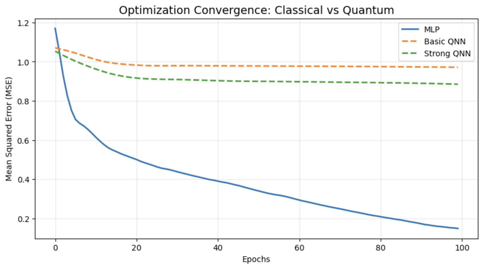
What the training curves show
 Enlarge figure ↗
The fixed-kernel QSVM outperformed both tested variational circuits, while the classical MLP retained the highest reported accuracy and F1. Early QNN loss plateaus motivate examining the optimization process directly.
Source: MatCom-2026 presentation, slides 4 and 6–9. These results describe predictive performance in the reported simulator experiment.
Future work
- Use repeated stratified splits to examine how stable the results are across different train/test partitions and four-component PCA representations.
- Measure gradient variance directly to investigate why the variational circuits plateau.
- Study shot noise and evaluate physical quantum hardware to extend the simulator comparison.
- Evaluate computational cost separately from classification accuracy when investigating quantum advantage.